Regression Trees

Name: Regression Tree

Introduction

Regression trees are very similar to standard decision trees, so we will just cover the notable differences in this article. If you haven't read the decision tree description yet, then read that one first. The model produced by the regression tree algorithm has exactly the same structure as a decision tree - that is, each node tests the value of an attribute in order to determine which branch to follow down the tree. However, the goal of regression trees is to predict a real number rather than a discrete class label. To this end, each leaf in a regression tree summarizes the target numbers that correspond to that segment of the data. This is usually either the mean or median target value of that segment/sub-population.

Like trees for classification, regression trees are a popular technique for knowledge discovery because the tree produced is very easy for humans to interpret. Whilst they are not very accurate by themselves, like classification trees their accuracy can be improved by learning a set of trees and combining them into an ensemble.

Learning Regression Trees

Again, the process of learning a regression trees is very similar to that of learning classification trees. The main difference is in how the "purity" of a segment is measured. Instead of trying to find segments with a strong majority of a discrete class label, regression trees look to find segments where the variance of target values is low. To that end, they tend to employ splitting metrics based on variance reduction. Both pre and post pruning strategies are employed in regression trees in order to prevent overfitting noise and spurious details in the training data.

Strengths

• Basic algorithm is reasonably simple to implement
• Considers attribute dependencies
• Simple for humans to interpret and understand how predictions are made
• Can be made more powerful by learning linear models at the leaves or by ensemble learning (both sacrifice some interpretability)

Weaknesses

• Suffers from the data fragmentation problem when there are nominal attributes with many distinct values
• Can produce large trees, which reduces interpretability
• Splitting criteria tend to be sensitive, and small changes in the data can result in large changes in the tree structure

 

Model interpretability: high

Common uses

Regression trees are usually employed when interpretability of the model is important and, of course, the target of interest is numeric (rather than discrete). Like decision trees, accuracy can be improved by various methods that learn ensembles of regression trees. However, these have the disadvantage of trading off that accuracy improvement for loss of interpretability in the final model. Interestingly, there is one modification of the single tree scenario that, in general, does improve accuracy whilst still retaining most of the interpretability of regression trees. Instead of predicting the mean or median of the target values of the instances that reach a given leaf, a multiple linear model can be fit to those instances. This sort of structure is called a model tree. The resulting model provides a piece-wise linear fit to non-linear target values. The decision structure of the tree can be followed to identify the segment that a new instance belongs to, and then the linear model's coefficients can be examined to see how the values of attributes within the segment relate to the target.

Configuration

The most important parameters for regression trees are essentially the same as those for classification trees. For pre-pruning approaches, this is tree depth. When post-pruning is applied, the default settings usually work well. Another parameter that also affects pre-pruning (although to a lesser extent than tree depth) is one that affects the minimum number of instances allowable at a leaf in the tree. This parameter can be more important in model trees where we need to ensure that there is enough data at a given leaf in the tree in order to build a stable linear regression.

Example

As we are talking about an algorithm for regression, we'll introduce a new dataset where the goal is to predict a real number. This dataset, called CPU, concerns the relative performance of computer processing power on the basis on the basis of a number of relevant characteristics. There are four attributes relating to main memory: cycle time (MYCT), minimum memory (MMIN), maximum memory (MMAX) and cache (CACH); there are also two attributes relating to channels: minimum channels (CHMIN) and maximum channels (CHMAX). Finally, there is the target: relative performance (PRP). There are 209 examples (rows) in this dataset, so we won't present them all here.

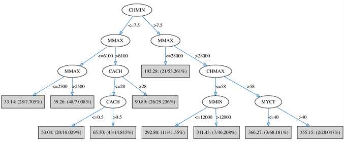
As was the case with the classification tree, the importance of attributes with respect to predicting the target is reflected in the level at which they are tested within the tree. So, in this case, the regression tree algorithm has chosen the CHMIN as the most predictive attribute with which to segment the data at the root. The next most important attribute - MMAX - is tested on both branches at the second layer of the tree. At the leaves of the tree (shaded rectangles) there are several pieces of information shown. The first number is the average of the target (PRP) values that reach the leaf in question. The first number in parentheses, to the left of the "/", is the number of training instances that reach the leaf in question; the second number is the percentage reduction in variance of the target values at the leaf, compared to that of the whole training set.